The power of craftsmanship
I am going through the fast.ai course “Practical Deep Learning for coders”, and I am liking it a lot. I might write something about it once I finish it, but long story short: if you are looking for something to get started on ML go ahead do it!
In the 4th lesson the focus is on building a ML model to tackle one of the great classics of the field: the MNIST dataset.
MNIST dataset: a timeless classic
There are a lot of resources about the MNIST dataset, here I’ll only mention that it is a huge dataset (it includes a total of 70k images) of hand-written digits. It has been built and used in the late 90s to run experiments with pattern recognition/computer vision models.
In the course, there is a deep dive into how to build a model on a simplified version of the dataset: only 3s and 7s are taken and a classifier is built. At the end of the chapter, one of the assignments for the students is to build a larger model to run on the full dataset, i.e. on all the numbers.
Start small and scale
I started out with the idea of generalizing to more digits what was done in the lesson for just two digits, which also means writing my own stuff instead of using built-in tools in the pytorch/fastai libraries. In particular, in the lesson an hand-made loss function was used:
def mnist_loss(predictions, targets):
    predictions = predictions.sigmoid()
    return torch.where(targets==1, 1-predictions, predictions).mean()
As mentioned above, the problem in the lesson is reduced to discriminate between 3s and 7s and it is implemented as detecting 3s, i.e. the idea is to train the model to answer the question “is this image a 3?” and since we are only using 3s and 7s, if it’s not a 3 it’s a 7.
The above loss function starts with taking the activations of the neurons and mapping them to values between 0 and 1 using the sigmoid function. The returned value is simply the actual prediction if the target is 0 and 1-prediction if the target is one. In this way high predictions are favoured when the target is one (i.e. the loss gets a 1-prediction) and low predictions are favoured when the target is 0. For the full explanation take a look here.
Wanting to simply generalize what was shown in the lesson I built a model with 10 outputs (one for each digit):
model1 = nn.Sequential(
    nn.Linear(28*28, 50),
    nn.ReLU(),
    nn.Linear(50,10),
)
For the loss function I simply expanded the above loss function to deal with the 10 predictions for each image. Here is what I came up with:
def myloss(predictions, target):

  predictions = predictions.sigmoid()

  target_encoded = torch.nn.functional.one_hot(target, 10)

  return torch.where( target_encoded==1, 1-predictions, predictions ).mean()
(I know, with just a bit more experience than I had when I wrote this, this is wrong. I will get there ![]() )
)
Here is what this function does:
- take the sigmoid of the predictions, in order to have all of them in the 0-1 range
- “one-hot” encode the target variable in a tensor with 10 values: all the elements in the vector are zero but the “target-th” element is 1: if the target for the given image is 5,
target_encodedis[0, 0, 0, 0, 0, 1, 0, 0, 0, 0]. - apply exactly the same logic as in the loss function used in the lesson
To have a practical example, let’s assume my model is processing an image of a 3 a 4 and a 0:
labels = [3,4,0]
t = torch.tensor(labels)
pred = torch.stack([
                  torch.tensor([-2, -3.5, -2.3, 3.5, -2.5, -2.1, -3.1, -3.4, -4, -3]),
                  torch.tensor([-2, -3.5, -2.3, -2.5, 3.5, -2.1, -3.1, -3.4, -4, -3]),
                  torch.tensor([3.5, -3.5, -2.3, -3.5, -2.5, -2.1, -3.1, -3.4, -4, -3]),
])
The above pred looks very similar to what it should look like for a good model: activations for the correct one-hot encoded labels are high for the correct digit (3rd in the first case, 4th in the second case and 0-th in the third case) and low elsewhere (i.e. units >0 and <0 respectively).
With the above numbers, myloss(pred[0], t[0]) gives a small value (tensor(0.0595)), while myloss(pred[1], t[0]) gives a higher value (tensor(0.2384)), as expected.
As a metric I used the accuracy, and hand-made accuracy of course:
def myaccuracy(predictions, targets):

  pred_nums = torch.argmax(predictions, axis=1)

  return (pred_nums==targets.T).float().mean()
Everything is set now, I just have to train the model and check how things go!
It’s hard to face the reality
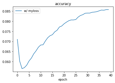
Not so well … The accuracy drops at the very beginning of the training, then starts growing, but the growth is slow and after 40 epochs (which is not much in general, but in the course models are usually trained for 5-10 epochs) it reaches the top at 8.5%.
As a comparison I trained a copy of the model with the built-in cross entropy function (i.e. the default loss function for multi-class classification problems) and here is what I get:
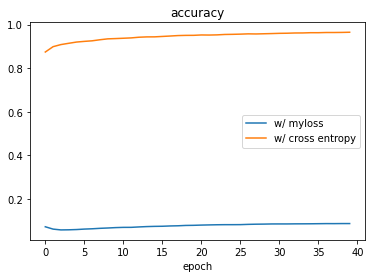
So there is nothing wrong with the model, the problem is with the loss function! And this is very weird, because myloss(...) behaves exactly as expected when testing it by hand!
I have been testing this a lot, but I could not get a good result (that’s how I got to use 40 epochs and a learning rate of 0.05, in case you were wondering ![]() ).
).
Since I couldn’t get my model to work, I simply decided to write a post on the fast.ai forum and move on with the course.
Study hard is always a good choice
In the next chapter of the course they introduce Cross Entropy, which is the real and proper generalization of the mnist_loss(...) loss function I was trying to generalize! To explain it in just a few words, it consists of 2 steps:
- take the softmax of the activations: this is a step forward compared to taking the sigmoid of the activations since not only it transforms the output in the 0-1 range, but it also transforms them in such a way that they add up to 1, making them basically probabilities!
- use the likelihood, which is the generalization of the
torch.where(...)step
As excited as I could be I fired up my Colab notebook again and implemented the wonderful cross entropy:
def myloss2(predictions, targets):

  sm = torch.softmax(predictions, dim=1)
  idx = tensor(range(len(targets)))

  return sm[idx, targets].mean()
Of course I ran straight to training the model using myloss2(...) as loss function and …
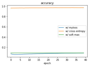
… oh no!
(face the reality, study hard,) repeat
Interestingly, using the right loss function does not help! The model still sucks!
Going further in the chapter, there is a nice session in which they talk about the importance of using logarithms when performing complicated calculations, and how this trick has been used since way earlier than computing loss functions in ML. But hey, don’t tell me, I am a physicist by education, I have a PhD and I have worked for years at CERN, so I know what logs are and how important they are! For sure such a minor detail which helps when performing huge computations is not needed for this very simple model that I am testing just to educate myself about Deep Learning … right??
Well, not really.
I implemented the log-based cross entropy, i.e. exactly the same as above but using log_softmax(...) and nll_loss(...) (which, despite the fancy name, is doing exactly the same as the last line of myloss2(...) and swapping the sign, as n stands for negative):
def myloss3(predictions, targets):

  sm = torch.log_softmax(predictions, dim=1)
  idx = tensor(range(len(targets)))

  return F.nll_loss(sm, targets.squeeze())
Let’s see if this works …
Long live the logarithms!
Here is the accuracy for the 4 models together:
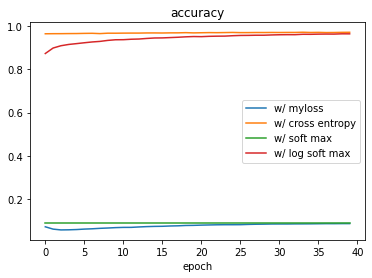
The model with the log-based cross entropy performs as good as the one with the pytorch native cross entropy!
This is a huge learning, I think: even if all the theory was correct and, if we leave out myloss(...), I was using the right cross entropy, still I could not get anything decent because of this practical issue of making calculations using huge numbers. Only using the logarithms to allow the computer to better handle the math allowed me to train the model properly and reach satisfactory results.
This relates to what Jeremy and Sylvain (the authors of the fast.ai book and MOOC) state later on in the course (Chapter 5) while talking about an image classification task:
Just a few years ago this was considered a very challenging task—but today, it’s far too easy!
These things look “far too easy” today because now we have means to train these models without too much effort (…), and indeed to write this post I could train 4 different models in just a few minutes, sitting at my desk and using GPUs. But these models are not “simple” per se, the very basic model I was training has plenty of parameters to train, and who knows how many other details which I am not even able to grasp at this stage are there.
These things are “far too easy” nowadays because they rely on all the breakthroughs and the steps forward that practitioner made in the field, and all of them count: the huge theoretical foundations, the minor refinements as well as all the things that help on a more practical level (and many examples of all of these are given in the course). I find all of this very exciting, since it really takes some kind of craftsmanshift to master any topic, it’s not enough to just read through the theory!